During the prototyping of the CRROPC, I’ve been writing software in C# to acquire signals from our photodetector, and process them into meaningful particle size distribution histograms. This allows us to see what happens when we put test aerosols through the instrument – we hope to see nice narrow peaks in our histogram corresponding to the scattering cross section of our particles (which can be linked to particle size)! In this post I’m going to briefly discuss the way the software is written, and how I can test it by simulating the signal from the photodetector. This is useful – test particles can be expensive, running them through the instrument can take time, and all the interacting subsystems of the instrument can generate confusing results in practice!

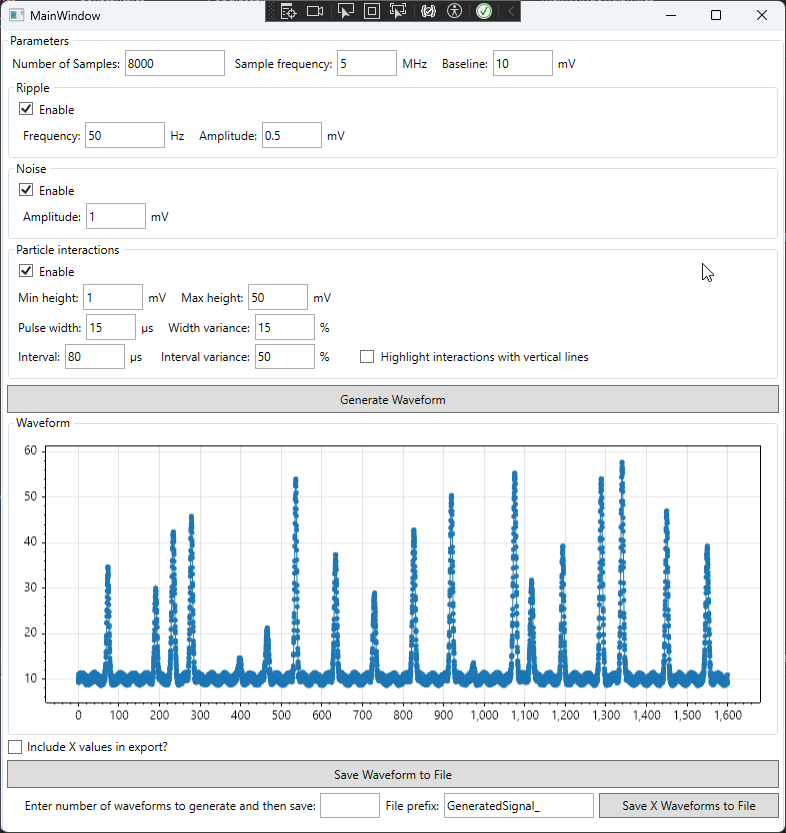
A quick summary of the signal generation process in our instrument: a photodetector outputs an analog voltage proportional to the light it detects (which has been scattered by particles, illuminated by a laser). This analog voltage is captured by an analog-to-digital converter (ADC), which for us is currently a Picoscope 4262. The Picoscope has custom programming libraries allowing us to load the captured signal into arbitrary custom code. This is what the raw voltage signal looks like:

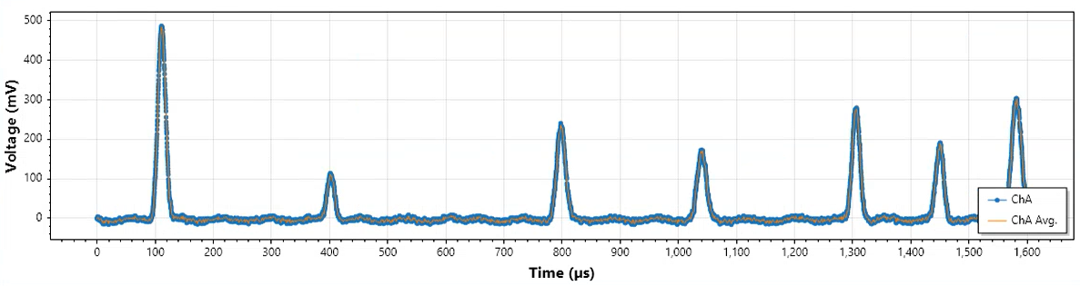
Each of those peaks in the data represents a probable particle crossing the laser beam. Within our data processing software, we will have a variety of different algorithms working on this signal – the primary example being an algorithm to detect peaks that stand out from the signal noise, and determine their amplitude (which is proportional to scattering cross section). Other algorithms might be calculating particle interaction times, voltage baseline level, signal noise – various parameters which either contribute to the scientific data, or indicate how well the instrument is functioning.

We can simulate the voltage signal quite easily, if we model each particle interaction as a Gaussian pulse (they’re not that far off). Additionally, various kinds of noise can be simulated. The steps might look something like this:

1. 1. Generate array of values with specified DC baseline
2. 2. Generate array of periodic sine wave noise with specified frequency, amplitude, etc. to represent 50 Hz mains noise, sum with base array
3. 3. Generate array of random noise values between specified amplitude range, sum with base array
4. 4. Generate array of Gaussian pulses with random values between a specified range for pulse interval, amplitude, pulse length, etc. Sum with base array
5. 5. Save to a .csv or other data structure

The software could be configured to load the simulated signal directly, rather than capture data from the ADC, but there is another way to insert the simulated signal without making any changes to the code – using an Arbitrary Waveform Generator (AWG).

Helpfully, we have a second Picoscope (a model 2204A) which is capable of AWG, and provides simple software for using it. We just load in a .csv file, and set the frequency/amplitude (some calculation might be needed to ensure the generated waveform exactly matches the simulated signal, if needed). This then generates an analog voltage that we can then measure with the ADC – so we can test more of the signal acquisition chain (albeit adding the random noise of the ADC to what would otherwise be an identical, repeating signal. However the ADC noise is substantially lower than the photodetector noise, so makes little difference in this case).

Our algorithms are now getting a consistent signal, and we can test what happens when we change them, without having to worry about the entire instrument!

This also leaves the door open to improved testing: we could simulate signals which stress-test the algorithms (e.g. what happens when two particles coincide and their pulses are hard to distinguish?), and we could write unit testing software to load in a large number of various simulated signals automatically – this helps find bugs, edge cases, etc.

Ben Rae